Chapter 6 Penalized Linear Regressions: A Simulation Experiment
6.1 Data Generating Process: Approximately Sparse
- Import libraries
R code
# No libraries requiered
Python code
import random
import numpy as np
import math
import matplotlib.pyplot as plt- To set seed
R code
set.seed(1)
n = 100
p = 400
Python code
random.seed(1)
n = 100
p = 400- To create variables
Z= runif(n)-1/2
W = matrix(runif(n*p)-1/2, n, p)
Z = np.random.uniform( low = 0 , high = 1 , size = n) - 1/2
W = ( np.random.uniform( low = 0 , high = 1 , size = n * p ) - 1/2 ).\
        reshape( n , p )
beta = 1/seq(1:p)^2 # approximately sparse beta
gX = exp(4*Z)+ W%*%beta # leading term nonlinear
X = cbind(Z, Z^2, Z^3, W ) # polynomials in Zs will be approximating exp(4*Z)
beta = ((1/ np.arange(1, p + 1 )) ** 2)
gX = np.exp( 4 * Z ) + (W @ beta)
X = np.concatenate( ( Z.reshape(Z.size, 1), Z.reshape(Z.size, 1) \
** 2, Z.reshape(Z.size, 1) ** 3, W ) , axis = 1 )- Generate \(Y\)
Y = gX + rnorm(n) #generate Y
mean = 0
sd = 1
Y = gX + np.random.normal( mean , sd, n )
#
#
#
#
#
plot(gX,Y, xlab="g(X)", ylab="Y", title("Y vs g(X)")) 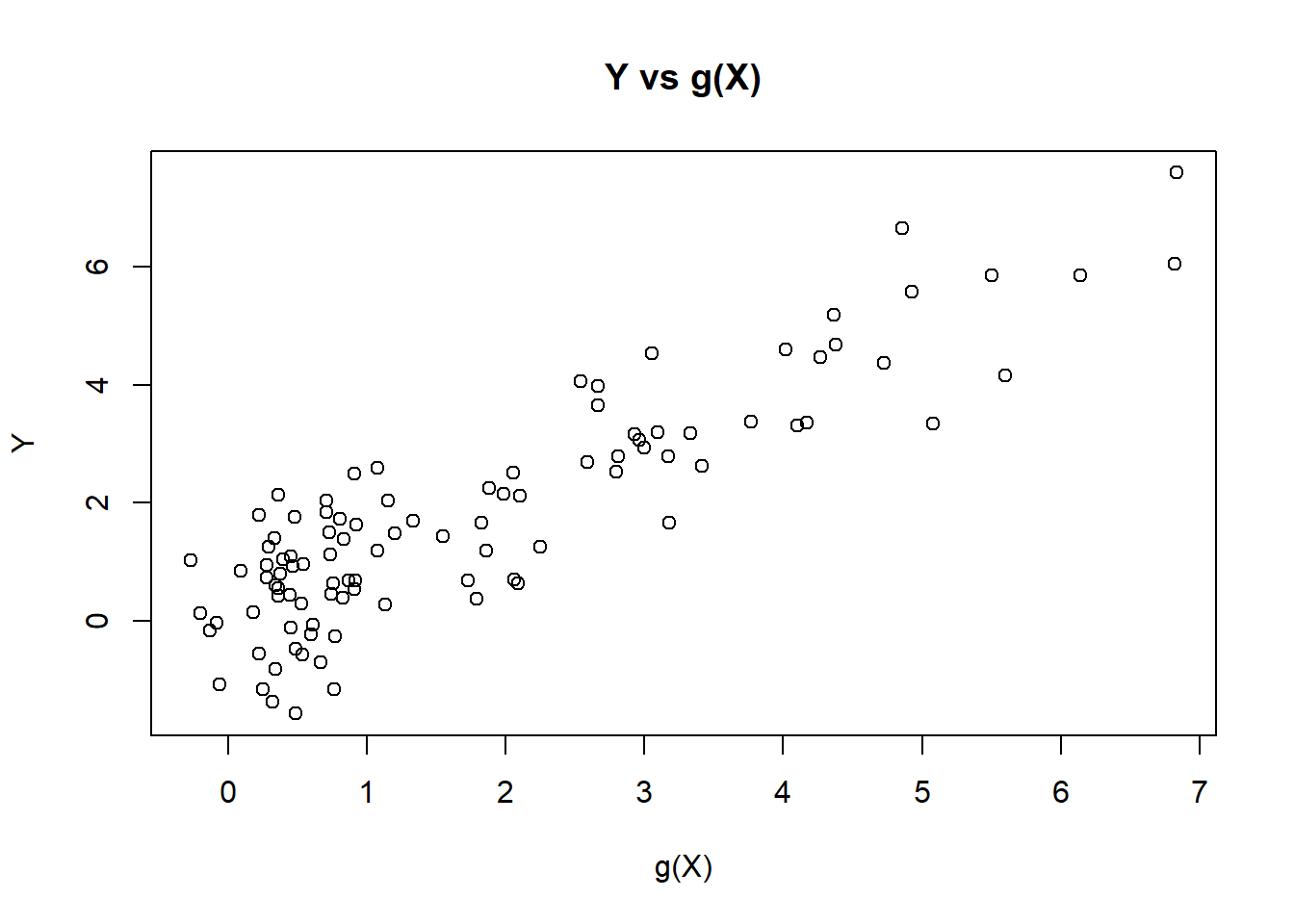
fig = plt.figure()
fig.suptitle('Y vs g(X)')
## Text(0.5, 0.98, 'Y vs g(X)')ax = fig.add_subplot(111)
plt.scatter( Y, gX)## <matplotlib.collections.PathCollection object at 0x000000002E7F3DF0>plt.xlabel('g(X)')## Text(0.5, 0, 'g(X)')plt.ylabel('Y')## Text(0, 0.5, 'Y')plt.show()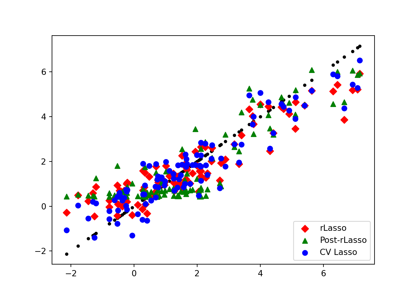
print( c("theoretical R2:", var(gX)/var(Y)))## [1] "theoretical R2:" "0.826881788964026"dim(X)## [1] 100 403
print( f"theoretical R2:, {np.var(gX) / np.var( Y )}" ) ## theoretical R2:, 0.8350134053252177X.shape## (100, 403)We use package Glmnet to carry out predictions using cross-validated lasso, ridge, and elastic net.
We should know that cv.glmnet function in r standarize X data by default. So, we have to standarize our data before the execution of sklearn package. The normalize parameter will help for this. However, the function cv.glamnet is also standarizing the Y variable and then unstadarize the coefficients from the regression. To do this with sklearn, we will standarize the Y variable before fitting with StandardScaler function. Finally, the r-function uses 10 folds by default so we will adjust our model to use \(cv=10\) ten folds.
The parameter \(l1_{ratio}\) corresponds to alpha in the glmnet R package while alpha corresponds to the lambda parameter in glmnet. Specifically, \(l1_{ratio} = 1\) is the lasso penalty. Currently, \(l1_{ratio} <= 0.01\) is not reliable, unless you supply your own sequence of alpha.
library(glmnet)
from sklearn.linear_model import LassoCV
from sklearn.preprocessing import StandardScaler
from sklearn.linear_model import RidgeCV, ElasticNetCV
import statsmodels.api as sm
fit.lasso.cv <- cv.glmnet(X, Y, family="gaussian", alpha=1) # family gaussian means that we'll be using square loss
fit.ridge <- cv.glmnet(X, Y, family="gaussian", alpha=0) # family gaussian means that we'll be using square loss
fit.elnet <- cv.glmnet(X, Y, family="gaussian", alpha=.5) # family gaussian means that we'll be using square loss
yhat.lasso.cv <- predict(fit.lasso.cv, newx = X) # predictions
yhat.ridge <- predict(fit.ridge, newx = X)
yhat.elnet <- predict(fit.elnet, newx = X)
MSE.lasso.cv <- summary(lm((gX-yhat.lasso.cv)^2~1))$coef[1:2] # report MSE and standard error for MSE for approximating g(X)
MSE.ridge <- summary(lm((gX-yhat.ridge)^2~1))$coef[1:2] # report MSE and standard error for MSE for approximating g(X)
MSE.elnet <- summary(lm((gX-yhat.elnet)^2~1))$coef[1:2] # report MSE and standard error for MSE for approximating g(X)
# Reshaping Y variable
Y_vec = Y.reshape( Y.size, 1)

# Scalar distribution
scaler = StandardScaler()
scaler.fit( Y_vec )
## StandardScaler()std_Y = scaler.transform( Y_vec )
# Regressions
fit_lasso_cv = LassoCV(cv = 10 , random_state = 0 , normalize = True ).fit( X, std_Y )## C:\Users\MSI-NB\ANACON~1\envs\TENSOR~2\lib\site-packages\sklearn\utils\validation.py:63: DataConversionWarning: A column-vector y was passed when a 1d array was expected. Please change the shape of y to (n_samples, ), for example using ravel().
## return f(*args, **kwargs)fit_ridge = ElasticNetCV( cv = 10 , normalize = True , random_state = 0 , l1_ratio = 0.0001 ).fit( X, std_Y )## C:\Users\MSI-NB\ANACON~1\envs\TENSOR~2\lib\site-packages\sklearn\utils\validation.py:63: DataConversionWarning: A column-vector y was passed when a 1d array was expected. Please change the shape of y to (n_samples, ), for example using ravel().
## return f(*args, **kwargs)fit_elnet = ElasticNetCV( cv = 10 , normalize = True , random_state = 0 , l1_ratio = 0.5, max_iter = 100000 ).fit( X, std_Y )
# Predictions## C:\Users\MSI-NB\ANACON~1\envs\TENSOR~2\lib\site-packages\sklearn\utils\validation.py:63: DataConversionWarning: A column-vector y was passed when a 1d array was expected. Please change the shape of y to (n_samples, ), for example using ravel().
## return f(*args, **kwargs)yhat_lasso_cv = scaler.inverse_transform( fit_lasso_cv.predict( X ) )
yhat_ridge = scaler.inverse_transform( fit_ridge.predict( X ) )
yhat_elnet = scaler.inverse_transform( fit_elnet.predict( X ) )
MSE_lasso_cv = sm.OLS( ((gX - yhat_lasso_cv)**2 ) , np.ones( yhat_lasso_cv.shape ) ).fit().summary2().tables[1].round(3)
MSE_ridge = sm.OLS( ((gX - yhat_ridge)**2 ) , np.ones( yhat_ridge.size ) ).fit().summary2().tables[1].round(3)
MSE_elnet = sm.OLS( ((gX - yhat_elnet)**2 ) , np.ones( yhat_elnet.size ) ).fit().summary2().tables[1].round(3)
# our coefficient of MSE_elnet are far from r outputHere we compute the lasso and ols post lasso using plug-in choices for penalty levels, using package hdm.
Rlasso functionality: it is searching the right set of regressors. This function was made for the case of p regressors and n observations where p >>>> n. It assumes that the error is i.i.d. The errors may be non-Gaussian or heteroscedastic.
The post lasso function makes OLS with the selected T regressors. To select those parameters, they use \(\lambda\) as variable to penalize Funny thing: the function rlasso was named like that because it is the “rigorous” Lasso. We find a Python code that tries to replicate the main function of hdm r-package. I was made by Max Huppertz.
His library is this repository. Download its repository and copy this folder to your site-packages folder. In my case it is located here C:-packages .
We need to install this package pip install multiprocess.
R code
library(hdm)
Python code
import hdmpyfit.rlasso <- rlasso(Y~X, post=FALSE) # lasso with plug-in penalty level
fit.rlasso.post <- rlasso(Y~X, post=TRUE) # post-lasso with plug-in penalty level
yhat.rlasso <- predict(fit.rlasso) #predict g(X) for values of X
yhat.rlasso.post <- predict(fit.rlasso.post) #predict g(X) for values of X
MSE.lasso <- summary(lm((gX-yhat.rlasso)^2~1))$coef[1:2] # report MSE and standard error for MSE for approximating g(X)
MSE.lasso.post <- summary(lm((gX-yhat.rlasso.post)^2~1))$coef[1:2] # report MSE and standard error for MSE for approximating g(X)
fit_rlasso = hdmpy.rlasso(X, Y, post = False)
fit_rlasso_post = hdmpy.rlasso(X, Y, post = True)
yhat_rlasso = Y - fit_rlasso.est['residuals'].reshape( Y.size, )
yhat_rlasso_post = Y - fit_rlasso_post.est['residuals'].reshape( Y.size , )
MSE_lasso = sm.OLS( ((gX - yhat_rlasso)**2 ) , np.ones( yhat_rlasso.size ) ).fit().summary2().tables[1].round(3)
MSE_lasso_post = sm.OLS( ((gX - yhat_rlasso_post)**2 ) , np.ones( yhat_rlasso_post.size ) ).fit().summary2().tables[1].round(3)Next we code up lava, which alternates the fitting of lasso and ridge
lava.predict<- function(X,Y, iter=5){
g1 = predict(rlasso(X, Y, post=F)) #lasso step fits "sparse part"
m1 = predict(glmnet(X, as.vector(Y-g1), family="gaussian", alpha=0, lambda =20),newx=X ) #ridge step fits the "dense" part
i=1
while(i<= iter) {
g1 = predict(rlasso(X, Y, post=F)) #lasso step fits "sparse part"
m1 = predict(glmnet(X, as.vector(Y-g1), family="gaussian", alpha=0, lambda =20),newx=X ); #ridge step fits the "dense" part
i = i+1 }
return(g1+m1);
}
def lava_predict( x, y, iteration = 5 ):
g1_rlasso = hdmpy.rlasso( x, y , post = False )
g1 = y - g1_rlasso.est['residuals'].reshape( g1_rlasso.est['residuals'].size, )
new_dep_var = y-g1
new_dep_var_vec = new_dep_var.reshape( new_dep_var.size, 1 )
# Scalar distribution
scaler = StandardScaler()
scaler.fit( new_dep_var_vec )
std_new_dep_var_vec = scaler.transform( new_dep_var_vec )
fit_ridge_m1 = ElasticNetCV( cv = 10 , normalize = True , random_state = 0 , l1_ratio = 0.0001, alphas = np.array([20]) ).fit( x, std_new_dep_var_vec )
m1 = scaler.inverse_transform( fit_ridge_m1.predict( x ) )
i = 1
while i <= iteration:
g1_rlasso = hdmpy.rlasso( x, y , post = False )
g1 = y - g1_rlasso.est['residuals'].reshape( g1_rlasso.est['residuals'].size, )
new_dep_var = y-g1
new_dep_var_vec = new_dep_var.reshape( new_dep_var.size, 1 )
# Scalar distribution
scaler = StandardScaler()
scaler.fit( new_dep_var_vec )
std_new_dep_var_vec = scaler.transform( new_dep_var_vec )
fit_ridge_m1 = ElasticNetCV( cv = 10 , normalize = True , random_state = 0 , l1_ratio = 0.0001, alphas = np.array([20]) ).fit( x, std_new_dep_var_vec )
m1 = scaler.inverse_transform( fit_ridge_m1.predict( x ) )
i = i + 1
return ( g1 + m1 )yhat.lava = lava.predict(X,Y)
MSE.lava <- summary(lm((gX-yhat.lava)^2~1))$coef[1:2]# report MSE and standard error for MSE for approximating g(X)
MSE.lava## [1] 0.16013551 0.02531404
yhat_lava = lava_predict( X, Y )## C:\Users\MSI-NB\ANACON~1\envs\TENSOR~2\lib\site-packages\sklearn\utils\validation.py:63: DataConversionWarning: A column-vector y was passed when a 1d array was expected. Please change the shape of y to (n_samples, ), for example using ravel().
## return f(*args, **kwargs)
## C:\Users\MSI-NB\ANACON~1\envs\TENSOR~2\lib\site-packages\sklearn\utils\validation.py:63: DataConversionWarning: A column-vector y was passed when a 1d array was expected. Please change the shape of y to (n_samples, ), for example using ravel().
##   return f(*args, **kwargs)
## C:\Users\MSI-NB\ANACON~1\envs\TENSOR~2\lib\site-packages\sklearn\utils\validation.py:63: DataConversionWarning: A column-vector y was passed when a 1d array was expected. Please change the shape of y to (n_samples, ), for example using ravel().
##   return f(*args, **kwargs)
## C:\Users\MSI-NB\ANACON~1\envs\TENSOR~2\lib\site-packages\sklearn\utils\validation.py:63: DataConversionWarning: A column-vector y was passed when a 1d array was expected. Please change the shape of y to (n_samples, ), for example using ravel().
##   return f(*args, **kwargs)
## C:\Users\MSI-NB\ANACON~1\envs\TENSOR~2\lib\site-packages\sklearn\utils\validation.py:63: DataConversionWarning: A column-vector y was passed when a 1d array was expected. Please change the shape of y to (n_samples, ), for example using ravel().
## return f(*args, **kwargs)
## C:\Users\MSI-NB\ANACON~1\envs\TENSOR~2\lib\site-packages\sklearn\utils\validation.py:63: DataConversionWarning: A column-vector y was passed when a 1d array was expected. Please change the shape of y to (n_samples, ), for example using ravel().
## return f(*args, **kwargs)MSE_lava = sm.OLS( ((gX - yhat_lava)**2 ) , np.ones( yhat_lava.size ) ).fit().summary2().tables[1].round(3)
MSE_lava## Coef. Std.Err. t P>|t| [0.025 0.975]
## const 0.253 0.043 5.916 0.0 0.168 0.338library(xtable)
table<- matrix(0, 6, 2)
table[1,1:2] <- MSE.lasso.cv
table[2,1:2] <- MSE.ridge
table[3,1:2] <- MSE.elnet
table[4,1:2] <- MSE.lasso
table[5,1:2] <- MSE.lasso.post
table[6,1:2] <- MSE.lava
colnames(table)<- c("MSA", "S.E. for MSA")
rownames(table)<- c("Cross-Validated Lasso", "Cross-Validated ridge","Cross-Validated elnet",
"Lasso","Post-Lasso","Lava")
tab <- xtable(table, digits =3)
print(tab,type="latex")## % latex table generated in R 4.0.4 by xtable 1.8-4 package
## % Wed Nov 24 12:24:54 2021
## \begin{table}[ht]
## \centering
## \begin{tabular}{rrr}
## \hline
## & MSA & S.E. for MSA \\
## \hline
## Cross-Validated Lasso & 0.367 & 0.061 \\
## Cross-Validated ridge & 2.384 & 0.370 \\
## Cross-Validated elnet & 0.399 & 0.064 \\
## Lasso & 0.148 & 0.027 \\
## Post-Lasso & 0.085 & 0.009 \\
## Lava & 0.160 & 0.025 \\
## \hline
## \end{tabular}
## \end{table}
import pandas as pd
table2 = np.zeros( (6, 2) )
table2[0, 0:] = MSE_lasso_cv.iloc[0, 0:2].to_list()
table2[1, 0:] = MSE_ridge.iloc[0, 0:2].to_list()
table2[2, 0:] = MSE_elnet.iloc[0, 0:2].to_list()
table2[3, 0:] = MSE_lasso.iloc[0, 0:2].to_list()
table2[4, 0:] = MSE_lasso_post.iloc[0, 0:2].to_list()
table2[5, 0:] = MSE_lava.iloc[0, 0:2].to_list()
table2_pandas = pd.DataFrame( table2, columns = [ "MSA","S.E. for MSA" ])
table2_pandas.index = [ "Cross-Validated Lasso",\
"Cross-Validated Ridge", "Cross-Validated elnet",\
"Lasso", "Post-Lasso", "Lava" ]
table2_pandas = table2_pandas.round(3)
table2_html = table2_pandas.to_html()
table2_pandas## MSA S.E. for MSA
## Cross-Validated Lasso 0.233 0.031
## Cross-Validated Ridge 3.098 0.492
## Cross-Validated elnet 0.476 0.056
## Lasso 0.253 0.043
## Post-Lasso 0.167 0.021
## Lava 0.253 0.043plot(gX, gX, pch=19, cex=1, ylab="predicted value", xlab="true g(X)")
points(gX, yhat.rlasso, col=2, pch=18, cex = 1.5 )
points(gX, yhat.rlasso.post, col=3, pch=17, cex = 1.2 )
points( gX, yhat.lasso.cv,col=4, pch=19, cex = 1.2 )
legend("bottomright",
legend = c("rLasso", "Post-rLasso", "CV Lasso"),col = c(2,3,4),
pch = c(18,17, 19),bty = "n",
pt.cex = 1.3, cex = 1.2,
text.col = "black", horiz = F ,inset = c(0.1, 0.1))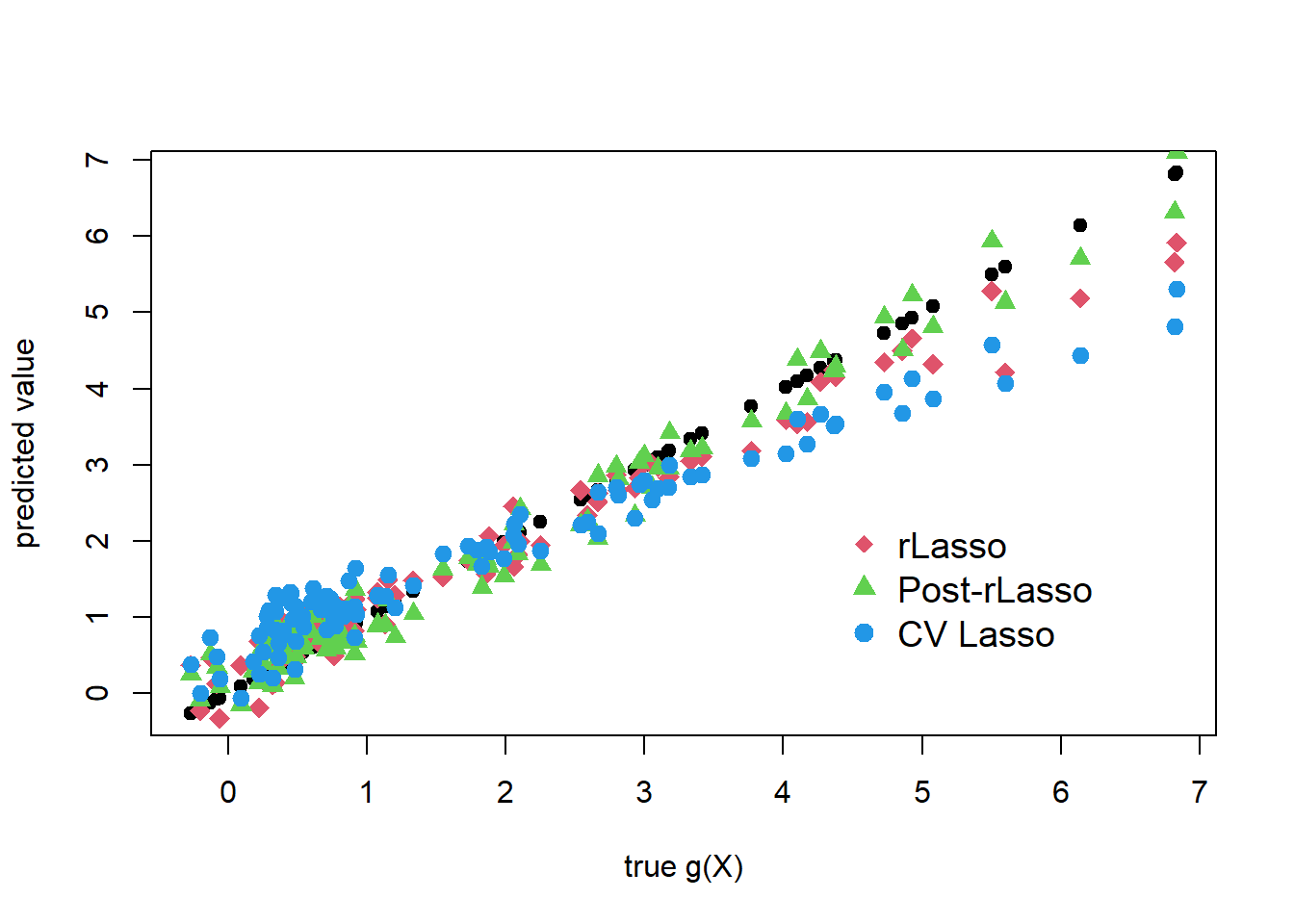
import matplotlib.pyplot as plt
fig = plt.figure()
ax1 = fig.add_subplot(111)
ax1.scatter( gX, gX , marker = '.', c = 'black' )## <matplotlib.collections.PathCollection object at 0x00000000055F2A90>ax1.scatter( gX, yhat_rlasso , marker = 'D' , c = 'red' , label = 'rLasso' )## <matplotlib.collections.PathCollection object at 0x00000000055F2F10>ax1.scatter( gX, yhat_rlasso_post , marker = '^' , c = 'green' , label = 'Post-rLasso')## <matplotlib.collections.PathCollection object at 0x0000000005606280>ax1.scatter( gX, yhat_lasso_cv , marker = 'o' , c = 'blue' , label = 'CV Lasso')## <matplotlib.collections.PathCollection object at 0x00000000056066D0>plt.legend(loc='lower right')## <matplotlib.legend.Legend object at 0x00000000055F2DF0>plt.show()
6.2 Data Generating Process: Approximately Sparse + Small Dense Part
R code
set.seed(1)
n = 100
p = 400
Z= runif(n)-1/2
W = matrix(runif(n*p)-1/2, n, p)
beta = rnorm(p)*.2 # dense beta
gX = exp(4*Z)+ W%*%beta # leading term nonlinear
X = cbind(Z, Z^2, Z^3, W ) # polynomials in Zs will be approximating exp(4*Z)
Y = gX + rnorm(n) #generate Y
Python code
n = 100
p = 400
Z = np.random.uniform( low = 0 , high = 1 , size = n) - 1/2
W = ( np.random.uniform( low = 0 , high = 1 , size = n * p ) - 1/2 ).\
reshape( n , p )
mean = 0
sd = 1
beta = ((np.random.normal( mean , sd, p )) * 0.2)
gX = np.exp( 4 * Z ) + (W @ beta)
X = np.concatenate( ( Z.reshape(Z.size, 1), Z.reshape(Z.size, 1) \
** 2, Z.reshape(Z.size, 1) ** 3, W ) , axis = 1 )
random.seed(2)
Y = gX + np.random.normal( mean , sd, n )#
#
#
#
#
#
#
plot(gX,Y, xlab="g(X)", ylab="Y") #plot V vs g(X)
# We use package Glmnet to carry out predictions using cross-validated lasso, ridge, and elastic net
fig = plt.figure()
fig.suptitle('Y vs g(X)')## Text(0.5, 0.98, 'Y vs g(X)')ax = fig.add_subplot(111)
plt.scatter( Y, gX)## <matplotlib.collections.PathCollection object at 0x0000000005B6FAC0>plt.xlabel('g(X)')## Text(0.5, 0, 'g(X)')plt.ylabel('Y')## Text(0, 0.5, 'Y')plt.show()
print( c("theoretical R2:", var(gX)/var(Y)))## [1] "theoretical R2:" "0.696687990094227"var(gX)/var(Y)## [,1]
## [1,] 0.696688
print( f"theoretical R2:, {np.var(gX) / np.var( Y )}" ) ## theoretical R2:, 0.9272949906911473np.var(gX) / np.var( Y ) #theoretical R-square in the simulation example## 0.9272949906911473library(glmnet)
# No librariesfit.lasso.cv <- cv.glmnet(X, Y, family="gaussian", alpha=1) # family gaussian means that we'll be using square loss
fit.ridge <- cv.glmnet(X, Y, family="gaussian", alpha=0) # family gaussian means that we'll be using square loss
fit.elnet <- cv.glmnet(X, Y, family="gaussian", alpha=.5) # family gaussian means that we'll be using square loss
yhat.lasso.cv <- predict(fit.lasso.cv, newx = X) # predictions
yhat.ridge <- predict(fit.ridge, newx = X)
yhat.elnet <- predict(fit.elnet, newx = X)
# Reshaping Y variable
Y_vec = Y.reshape( Y.size, 1)
# Scalar distribution
scaler = StandardScaler()
scaler.fit( Y_vec )## StandardScaler()std_Y = scaler.transform( Y_vec )
# Regressions
fit_lasso_cv = LassoCV(cv = 10 , random_state = 0 , normalize = True ).fit( X, std_Y )## C:\Users\MSI-NB\ANACON~1\envs\TENSOR~2\lib\site-packages\sklearn\utils\validation.py:63: DataConversionWarning: A column-vector y was passed when a 1d array was expected. Please change the shape of y to (n_samples, ), for example using ravel().
## return f(*args, **kwargs)fit_ridge = ElasticNetCV( cv = 10 , normalize = True , random_state = 0 , l1_ratio = 0.0001 ).fit( X, std_Y )## C:\Users\MSI-NB\ANACON~1\envs\TENSOR~2\lib\site-packages\sklearn\utils\validation.py:63: DataConversionWarning: A column-vector y was passed when a 1d array was expected. Please change the shape of y to (n_samples, ), for example using ravel().
## return f(*args, **kwargs)fit_elnet = ElasticNetCV( cv = 10 , normalize = True , random_state = 0 , l1_ratio = 0.5, max_iter = 100000 ).fit( X, std_Y )
# Predictions## C:\Users\MSI-NB\ANACON~1\envs\TENSOR~2\lib\site-packages\sklearn\utils\validation.py:63: DataConversionWarning: A column-vector y was passed when a 1d array was expected. Please change the shape of y to (n_samples, ), for example using ravel().
## return f(*args, **kwargs)yhat_lasso_cv = scaler.inverse_transform( fit_lasso_cv.predict( X ) )
yhat_ridge = scaler.inverse_transform( fit_ridge.predict( X ) )
yhat_elnet = scaler.inverse_transform( fit_elnet.predict( X ) )MSE.lasso.cv <- summary(lm((gX-yhat.lasso.cv)^2~1))$coef[1:2] # report MSE and standard error for MSE for approximating g(X)
MSE.ridge <- summary(lm((gX-yhat.ridge)^2~1))$coef[1:2] # report MSE and standard error for MSE for approximating g(X)
MSE.elnet <- summary(lm((gX-yhat.elnet)^2~1))$coef[1:2] # report MSE and standard error for MSE for approximating g(X)
MSE_lasso_cv = sm.OLS( ((gX - yhat_lasso_cv)**2 ) , np.ones( yhat_lasso_cv.shape ) ).fit().summary2().tables[1].round(3)
MSE_ridge = sm.OLS( ((gX - yhat_ridge)**2 ) , np.ones( yhat_ridge.size ) ).fit().summary2().tables[1].round(3)
MSE_elnet = sm.OLS( ((gX - yhat_elnet)**2 ) , np.ones( yhat_elnet.size ) ).fit().summary2().tables[1].round(3)
# our coefficient of MSE_elnet are far from r outputfit.rlasso <- rlasso(Y~X, post=FALSE) # lasso with plug-in penalty level
fit.rlasso.post <- rlasso(Y~X, post=TRUE) # post-lasso with plug-in penalty level
yhat.rlasso <- predict(fit.rlasso) #predict g(X) for values of X
yhat.rlasso.post <- predict(fit.rlasso.post) #predict g(X) for values of X
MSE.lasso <- summary(lm((gX-yhat.rlasso)^2~1))$coef[1:2] # report MSE and standard error for MSE for approximating g(X)
MSE.lasso.post <- summary(lm((gX-yhat.rlasso.post)^2~1))$coef[1:2] # report MSE and standard error for MSE for approximating g(X)
fit_rlasso = hdmpy.rlasso(X, Y, post = False)
fit_rlasso_post = hdmpy.rlasso(X, Y, post = True)

yhat_rlasso = Y - fit_rlasso.est['residuals'].reshape( Y.size,  )
yhat_rlasso_post = Y - fit_rlasso_post.est['residuals'].reshape( Y.size ,  )

MSE_lasso = sm.OLS( ((gX - yhat_rlasso)**2 ) , np.ones( yhat_rlasso.size )  ).fit().summary2().tables[1].round(3)
MSE_lasso_post = sm.OLS( ((gX - yhat_rlasso_post)**2 ) , np.ones( yhat_rlasso_post.size ) ).fit().summary2().tables[1].round(3)lava.predict<- function(X,Y, iter=5){
g1 = predict(rlasso(X, Y, post=F)) #lasso step fits "sparse part"
m1 = predict(glmnet(X, as.vector(Y-g1), family="gaussian", alpha=0, lambda =20),newx=X ) #ridge step fits the "dense" part
i=1
while(i<= iter) {
g1 = predict(rlasso(X, Y, post=F)) #lasso step fits "sparse part"
m1 = predict(glmnet(X, as.vector(Y-g1), family="gaussian", alpha=0, lambda =20),newx=X ); #ridge step fits the "dense" part
i = i+1 }
return(g1+m1);
}
def lava_predict( x, y, iteration = 5 ):

    g1_rlasso = hdmpy.rlasso( x, y , post = False )
    g1 = y - g1_rlasso.est['residuals'].reshape( g1_rlasso.est['residuals'].size, )

    new_dep_var = y-g1
    new_dep_var_vec = new_dep_var.reshape( new_dep_var.size, 1 )

    # Scalar distribution
    scaler = StandardScaler()
    scaler.fit( new_dep_var_vec )
    std_new_dep_var_vec = scaler.transform( new_dep_var_vec )

    fit_ridge_m1 = ElasticNetCV( cv = 10 , normalize = True , random_state = 0 , l1_ratio = 0.0001, alphas = np.array([20]) ).fit( x, std_new_dep_var_vec )
    m1 = scaler.inverse_transform( fit_ridge_m1.predict( x ) )

    i = 1
    while i <= iteration:

        g1_rlasso = hdmpy.rlasso( x, y , post = False )
        g1 = y - g1_rlasso.est['residuals'].reshape( g1_rlasso.est['residuals'].size, )

        new_dep_var = y-g1
        new_dep_var_vec = new_dep_var.reshape( new_dep_var.size, 1 )

        # Scalar distribution
        scaler = StandardScaler()
        scaler.fit( new_dep_var_vec )
        std_new_dep_var_vec = scaler.transform( new_dep_var_vec )

        fit_ridge_m1 = ElasticNetCV( cv = 10 , normalize = True , random_state = 0 , l1_ratio = 0.0001, alphas = np.array([20]) ).fit( x, std_new_dep_var_vec )
        m1 = scaler.inverse_transform( fit_ridge_m1.predict( x ) )

        i = i + 1

    return ( g1 + m1 )
yhat.lava = lava.predict(X,Y)
MSE.lava <- summary(lm((gX-yhat.lava)^2~1))$coef[1:2] # report MSE and standard error for MSE for approximating g(X)
yhat_lava = lava_predict( X, Y )## C:\Users\MSI-NB\ANACON~1\envs\TENSOR~2\lib\site-packages\sklearn\utils\validation.py:63: DataConversionWarning: A column-vector y was passed when a 1d array was expected. Please change the shape of y to (n_samples, ), for example using ravel().
## return f(*args, **kwargs)
## C:\Users\MSI-NB\ANACON~1\envs\TENSOR~2\lib\site-packages\sklearn\utils\validation.py:63: DataConversionWarning: A column-vector y was passed when a 1d array was expected. Please change the shape of y to (n_samples, ), for example using ravel().
##   return f(*args, **kwargs)
## C:\Users\MSI-NB\ANACON~1\envs\TENSOR~2\lib\site-packages\sklearn\utils\validation.py:63: DataConversionWarning: A column-vector y was passed when a 1d array was expected. Please change the shape of y to (n_samples, ), for example using ravel().
##   return f(*args, **kwargs)
## C:\Users\MSI-NB\ANACON~1\envs\TENSOR~2\lib\site-packages\sklearn\utils\validation.py:63: DataConversionWarning: A column-vector y was passed when a 1d array was expected. Please change the shape of y to (n_samples, ), for example using ravel().
##   return f(*args, **kwargs)
## C:\Users\MSI-NB\ANACON~1\envs\TENSOR~2\lib\site-packages\sklearn\utils\validation.py:63: DataConversionWarning: A column-vector y was passed when a 1d array was expected. Please change the shape of y to (n_samples, ), for example using ravel().
## return f(*args, **kwargs)
## C:\Users\MSI-NB\ANACON~1\envs\TENSOR~2\lib\site-packages\sklearn\utils\validation.py:63: DataConversionWarning: A column-vector y was passed when a 1d array was expected. Please change the shape of y to (n_samples, ), for example using ravel().
## return f(*args, **kwargs)MSE_lava = sm.OLS( ((gX - yhat_lava)**2 ) , np.ones( yhat_lava.size ) ).fit().summary2().tables[1].round(3)table<- matrix(0, 6, 2)
table[1,1:2] <- MSE.lasso.cv
table[2,1:2] <- MSE.ridge
table[3,1:2] <- MSE.elnet
table[4,1:2] <- MSE.lasso
table[5,1:2] <- MSE.lasso.post
table[6,1:2] <- MSE.lava
colnames(table)<- c("MSA", "S.E. for MSA")
rownames(table)<- c("Cross-Validated Lasso", "Cross-Validated ridge","Cross-Validated elnet","Lasso","Post-Lasso","Lava")
tab <- xtable(table, digits =3)
print(tab,type="latex") # set type="latex" for printing table in LaTeX## % latex table generated in R 4.0.4 by xtable 1.8-4 package
## % Wed Nov 24 12:26:46 2021
## \begin{table}[ht]
## \centering
## \begin{tabular}{rrr}
## \hline
## & MSA & S.E. for MSA \\
## \hline
## Cross-Validated Lasso & 1.932 & 0.291 \\
## Cross-Validated ridge & 3.411 & 0.494 \\
## Cross-Validated elnet & 1.825 & 0.252 \\
## Lasso & 0.964 & 0.120 \\
## Post-Lasso & 1.597 & 0.207 \\
## Lava & 0.661 & 0.072 \\
## \hline
## \end{tabular}
## \end{table}tab## % latex table generated in R 4.0.4 by xtable 1.8-4 package
## % Wed Nov 24 12:26:46 2021
## \begin{table}[ht]
## \centering
## \begin{tabular}{rrr}
## \hline
## & MSA & S.E. for MSA \\
## \hline
## Cross-Validated Lasso & 1.932 & 0.291 \\
## Cross-Validated ridge & 3.411 & 0.494 \\
## Cross-Validated elnet & 1.825 & 0.252 \\
## Lasso & 0.964 & 0.120 \\
## Post-Lasso & 1.597 & 0.207 \\
## Lava & 0.661 & 0.072 \\
## \hline
## \end{tabular}
## \end{table}
table2 = np.zeros( (6, 2) )

table2[0, 0:] = MSE_lasso_cv.iloc[0, 0:2].to_list()
table2[1, 0:] = MSE_ridge.iloc[0, 0:2].to_list()
table2[2, 0:] = MSE_elnet.iloc[0, 0:2].to_list()
table2[3, 0:] = MSE_lasso.iloc[0, 0:2].to_list()
table2[4, 0:] = MSE_lasso_post.iloc[0, 0:2].to_list()
table2[5, 0:] = MSE_lava.iloc[0, 0:2].to_list()


table2_pandas = pd.DataFrame( table2, columns = [ "MSA","S.E. for MSA" ])
table2_pandas.index = [ "Cross-Validated Lasso",\
                       "Cross-Validated Ridge", "Cross-Validated elnet",\
                       "Lasso", "Post-Lasso", "Lava" ]
table2_pandas = table2_pandas.round(3)
table2_html = table2_pandas.to_html()
table2_pandas
## MSA S.E. for MSA
## Cross-Validated Lasso 0.681 0.094
## Cross-Validated Ridge 3.897 0.559
## Cross-Validated elnet 0.815 0.106
## Lasso 0.854 0.127
## Post-Lasso 1.127 0.137
## Lava 0.852 0.126plot(gX, gX, pch=19, cex=1, ylab="predicted value", xlab="true g(X)")
points(gX, yhat.rlasso, col=2, pch=18, cex = 1.5 )
points(gX, yhat.elnet, col=3, pch=17, cex = 1.2 )
points(gX, yhat.lava, col=4, pch=19, cex = 1.2 )
legend("bottomright",
legend = c("rLasso", "Elnet", "Lava"),
col = c(2,3,4),
pch = c(18,17, 19),
bty = "n",
pt.cex = 1.3,
cex = 1.2,
text.col = "black",
horiz = F ,
inset = c(0.1, 0.1))
fig = plt.figure()

ax1 = fig.add_subplot(111)
ax1.scatter( gX, gX , marker = '.', c = 'black' )
## <matplotlib.collections.PathCollection object at 0x0000000005D140D0>ax1.scatter( gX, yhat_rlasso , marker = 'D' , c = 'red' , label = 'rLasso' )## <matplotlib.collections.PathCollection object at 0x0000000005D14520>ax1.scatter( gX, yhat_rlasso_post , marker = '^' , c = 'green' , label = 'Post-rLasso')## <matplotlib.collections.PathCollection object at 0x0000000005D14940>ax1.scatter( gX, yhat_lasso_cv , marker = 'o' , c = 'blue' , label = 'CV Lasso')## <matplotlib.collections.PathCollection object at 0x0000000005D14D60>plt.legend(loc='lower right')## <matplotlib.legend.Legend object at 0x0000000005D14D30>plt.show()