Chapter 21 A Simple Example of Properties of IV estimator when Instruments are Weak
Simulation Design
# Simulation Design

library(hdm)
set.seed(1)
B= 10000 # trials
IVEst = rep(0, B)
n=100
beta = .25   # .2 weak IV
#beta = 1   #   1 strong IV


U =  rnorm(n)
Z = rnorm(n)  #generate instrument
D = beta*Z + U  #generate endogenougs variable
Y =  D+ U  # the true causal effect is 1


summary(lm(D~Z))  # first stage is very weak here
##
## Call:
## lm(formula = D ~ Z)
##
## Residuals:
## Min 1Q Median 3Q Max
## -2.32416 -0.60361 0.00536 0.58305 2.29316
##
## Coefficients:
## Estimate Std. Error t value Pr(>|t|)
## (Intercept) 0.10885 0.09035 1.205 0.23118
## Z 0.24907 0.09472 2.629 0.00993 **
## ---
## Signif. codes: 0 '***' 0.001 '**' 0.01 '*' 0.05 '.' 0.1 ' ' 1
##
## Residual standard error: 0.9028 on 98 degrees of freedom
## Multiple R-squared: 0.0659, Adjusted R-squared: 0.05637
## F-statistic: 6.914 on 1 and 98 DF, p-value: 0.009931
import hdmpy
import numpy as np
import random
import statsmodels.api as sm
import matplotlib.pyplot as plt
import numpy as np
from matplotlib import colors
from statsmodels.sandbox.regression.gmm import IV2SLS
import numpy as np
import seaborn as sns
from scipy import stats
import matplotlib.pyplot as plt
import warnings
warnings.filterwarnings("ignore")

# Simulation Design

# Set seed
np.random.seed(0)
B = 1000
IVEst = np.zeros( B )
n = 100
beta = .25

mean = 0
sd = 1

U = np.random.normal( mean , sd, n ).reshape( n, 1 )
Z = np.random.normal( mean , sd, n ).reshape( n, 1 )
D = beta*Z + U
Y = D + U

mod = sm.OLS(D, sm.add_constant(Z))    # Describe model
res = mod.fit()
print(res.summary())
## OLS Regression Results
## ==============================================================================
## Dep. Variable: y R-squared: 0.121
## Model: OLS Adj. R-squared: 0.112
## Method: Least Squares F-statistic: 13.47
## Date: Wed, 24 Nov 2021 Prob (F-statistic): 0.000395
## Time: 16:39:05 Log-Likelihood: -142.05
## No. Observations: 100 AIC: 288.1
## Df Residuals: 98 BIC: 293.3
## Df Model: 1
## Covariance Type: nonrobust
## ==============================================================================
## coef std err t P>|t| [0.025 0.975]
## ------------------------------------------------------------------------------
## const 0.0509 0.101 0.501 0.617 -0.151 0.252
## x1 0.3588 0.098 3.670 0.000 0.165 0.553
## ==============================================================================
## Omnibus: 0.445 Durbin-Watson: 1.865
## Prob(Omnibus): 0.801 Jarque-Bera (JB): 0.594
## Skew: 0.041 Prob(JB): 0.743
## Kurtosis: 2.632 Cond. No. 1.09
## ==============================================================================
##
## Notes:
## [1] Standard Errors assume that the covariance matrix of the errors is correctly specified.summary(tsls(x=NULL, d=D, y=Y, z=Z)) ### [1] "Estimates and Significance Testing from from tsls"
## Estimate Std. Error t value p value
## d1 0.99626 0.38173 2.610 0.00906 **
## (Intercept) 0.10926 0.09824 1.112 0.26608
## ---
## Signif. codes: 0 '***' 0.001 '**' 0.01 '*' 0.05 '.' 0.1 ' ' 1
IV = IV2SLS(Y, D, sm.add_constant(Z))
IV_res = IV.fit()
print(IV_res.summary())
## IV2SLS Regression Results
## ==============================================================================
## Dep. Variable: y R-squared: 0.892
## Model: IV2SLS Adj. R-squared: 0.891
## Method: Two Stage F-statistic: nan
## Least Squares Prob (F-statistic): nan
## Date: Wed, 24 Nov 2021
## Time: 16:39:05
## No. Observations: 100
## Df Residuals: 99
## Df Model: 1
## ==============================================================================
## coef std err t P>|t| [0.025 0.975]
## ------------------------------------------------------------------------------
## x1 1.3230 0.180 7.365 0.000 0.967 1.679
## ==============================================================================
## Omnibus: 0.446 Durbin-Watson: 1.864
## Prob(Omnibus): 0.800 Jarque-Bera (JB): 0.595
## Skew: 0.044 Prob(JB): 0.743
## Kurtosis: 2.633 Cond. No. 1.00
## ==============================================================================Note that the instrument is weak here (contolled by \(\beta\)) – the t-stat is less than 4.
21.1 Run 1000 trials to evaluate distribution of the IV estimator
# Simulation Design

set.seed(1)
B= 10000 # trials
IVEst = rep(0, B)

for(i in 1:B){
U =  rnorm(n)
Z = rnorm(n)  #generate instrument
D = beta*Z + U  #generate endogenougs variable
Y =  D+ U  # the true causal effect is 1
IVEst[i] = coef(tsls(x=NULL, d=D, y=Y, z=Z))[1,1]
}
# Simulation design

# Set seed
np.random.seed(0)
B = 1000 # Trials
IVEst = np.zeros( B )

for i in range( 0, B ):
    U = np.random.normal( mean , sd, n ).reshape( n, 1 )
    Z = np.random.normal( mean , sd, n ).reshape( n, 1 )
    D = beta*Z + U
    Y = D + U

    IV = IV2SLS(Y, D, sm.add_constant(Z))
    IV_res = IV.fit()

    IVEst[ i ] = IV_res.summary2().tables[1]["Coef."][0]
21.2 Plot the Actual Distribution against the Normal Approximation (based on Strong Instrument Assumption)
plot(density(IVEst-1, n=1000, from=-5, to=5),col=4, xlim= c(-5, 5),
     xlab= "IV Estimator -True Effect", main="Actual Distribution vs Gaussian")

val=seq(-5, 5, by=.05)
var = (1/beta^2)*(1/100) # theoretical variance of IV
sd = sqrt(var)
lines(val, dnorm(val, sd=sd), col=2, lty=2)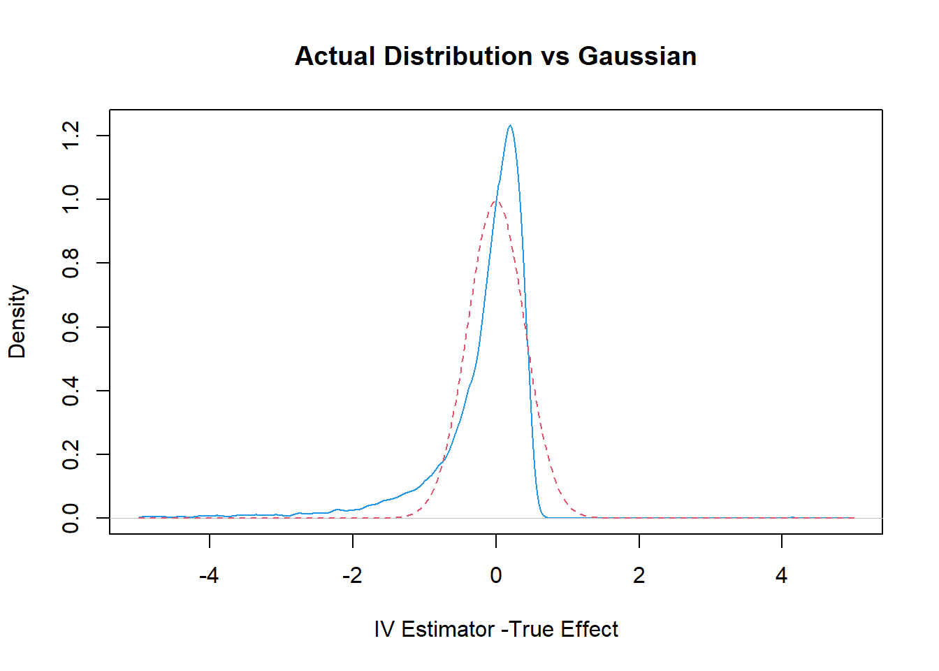
rejection.frequency = sum(( abs(IVEst-1)/sd > 1.96))/B
val = np.arange(-5,5.5,0.05)
var = (1/beta**2)*(1/100)   # theoretical variance of IV
sd = np.sqrt(var)

normal_dist = np.random.normal(0,sd,val.shape[0])

# plotting both distibutions on the same figure
fig = sns.kdeplot(IVEst-1, shade=True, color="r")
fig = sns.kdeplot(normal_dist, shade=True, color="b")

plt.title("Actual Distribution vs Gaussian")
## Text(0.5, 1.0, 'Actual Distribution vs Gaussian')plt.xlabel('IV Estimator -True Effect')## Text(0.5, 0, 'IV Estimator -True Effect')plt.xlim(-5,5)
## (-5.0, 5.0)cat(c("Rejection Frequency is ",
rejection.frequency, " while we expect it to be .05"))## Rejection Frequency is 0.1401 while we expect it to be .05
rejection_frequency = np.sum(( np.abs(IVEst-1)/sd > 1.96))/B
print( f"Rejection Frequency is {rejection_frequency} ,while we expect it to be .05")
## Rejection Frequency is 0.079 ,while we expect it to be .0521.3 Some Help Functions
help(tsls)
help(IV2SLS)## Help on class IV2SLS in module statsmodels.sandbox.regression.gmm:
##
## class IV2SLS(statsmodels.base.model.LikelihoodModel)
## | IV2SLS(endog, exog, instrument=None)
## |
## | Instrumental variables estimation using Two-Stage Least-Squares (2SLS)
## |
## |
## | Parameters
## | ----------
## | endog : ndarray
## | Endogenous variable, 1-dimensional or 2-dimensional array nobs by 1
## | exog : ndarray
## | Explanatory variables, 1-dimensional or 2-dimensional array nobs by k
## | instrument : ndarray
## | Instruments for explanatory variables. Must contain both exog
## | variables that are not being instrumented and instruments
## |
## | Notes
## | -----
## | All variables in exog are instrumented in the calculations. If variables
## | in exog are not supposed to be instrumented, then these variables
## | must also to be included in the instrument array.
## |
## | Degrees of freedom in the calculation of the standard errors uses
## | `df_resid = (nobs - k_vars)`.
## | (This corresponds to the `small` option in Stata's ivreg2.)
## |
## | Method resolution order:
## | IV2SLS
## | statsmodels.base.model.LikelihoodModel
## | statsmodels.base.model.Model
## | builtins.object
## |
## | Methods defined here:
## |
## | __init__(self, endog, exog, instrument=None)
## | Initialize self. See help(type(self)) for accurate signature.
## |
## | fit(self)
## | estimate model using 2SLS IV regression
## |
## | Returns
## | -------
## | results : instance of RegressionResults
## | regression result
## |
## | Notes
## | -----
## | This returns a generic RegressioResults instance as defined for the
## | linear models.
## |
## | Parameter estimates and covariance are correct, but other results
## | have not been tested yet, to see whether they apply without changes.
## |
## | initialize(self)
## | Initialize (possibly re-initialize) a Model instance.
## |
## | For example, if the the design matrix of a linear model changes then
## | initialized can be used to recompute values using the modified design
## | matrix.
## |
## | predict(self, params, exog=None)
## | Return linear predicted values from a design matrix.
## |
## | Parameters
## | ----------
## | exog : array_like
## | Design / exogenous data
## | params : array_like, optional after fit has been called
## | Parameters of a linear model
## |
## | Returns
## | -------
## | An array of fitted values
## |
## | Notes
## | -----
## | If the model as not yet been fit, params is not optional.
## |
## | whiten(self, X)
## | Not implemented
## |
## | ----------------------------------------------------------------------
## | Methods inherited from statsmodels.base.model.LikelihoodModel:
## |
## | hessian(self, params)
## | The Hessian matrix of the model.
## |
## | Parameters
## | ----------
## | params : ndarray
## | The parameters to use when evaluating the Hessian.
## |
## | Returns
## | -------
## | ndarray
## | The hessian evaluated at the parameters.
## |
## | information(self, params)
## | Fisher information matrix of model.
## |
## | Returns -1 * Hessian of the log-likelihood evaluated at params.
## |
## | Parameters
## | ----------
## | params : ndarray
## | The model parameters.
## |
## | loglike(self, params)
## | Log-likelihood of model.
## |
## | Parameters
## | ----------
## | params : ndarray
## | The model parameters used to compute the log-likelihood.
## |
## | Notes
## | -----
## | Must be overridden by subclasses.
## |
## | score(self, params)
## | Score vector of model.
## |
## | The gradient of logL with respect to each parameter.
## |
## | Parameters
## | ----------
## | params : ndarray
## | The parameters to use when evaluating the Hessian.
## |
## | Returns
## | -------
## | ndarray
## | The score vector evaluated at the parameters.
## |
## | ----------------------------------------------------------------------
## | Class methods inherited from statsmodels.base.model.Model:
## |
## | from_formula(formula, data, subset=None, drop_cols=None, *args, **kwargs) from builtins.type
## | Create a Model from a formula and dataframe.
## |
## | Parameters
## | ----------
## | formula : str or generic Formula object
## | The formula specifying the model.
## | data : array_like
## | The data for the model. See Notes.
## | subset : array_like
## | An array-like object of booleans, integers, or index values that
## | indicate the subset of df to use in the model. Assumes df is a
## | `pandas.DataFrame`.
## | drop_cols : array_like
## | Columns to drop from the design matrix. Cannot be used to
## | drop terms involving categoricals.
## | *args
## | Additional positional argument that are passed to the model.
## | **kwargs
## | These are passed to the model with one exception. The
## | ``eval_env`` keyword is passed to patsy. It can be either a
## | :class:`patsy:patsy.EvalEnvironment` object or an integer
## | indicating the depth of the namespace to use. For example, the
## | default ``eval_env=0`` uses the calling namespace. If you wish
## | to use a "clean" environment set ``eval_env=-1``.
## |
## | Returns
## | -------
## | model
## | The model instance.
## |
## | Notes
## | -----
## | data must define __getitem__ with the keys in the formula terms
## | args and kwargs are passed on to the model instantiation. E.g.,
## | a numpy structured or rec array, a dictionary, or a pandas DataFrame.
## |
## | ----------------------------------------------------------------------
## | Readonly properties inherited from statsmodels.base.model.Model:
## |
## | endog_names
## | Names of endogenous variables.
## |
## | exog_names
## | Names of exogenous variables.
## |
## | ----------------------------------------------------------------------
## | Data descriptors inherited from statsmodels.base.model.Model:
## |
## | __dict__
## | dictionary for instance variables (if defined)
## |
## | __weakref__
## | list of weak references to the object (if defined)help(density)
help(sns.kdeplot)## Help on function kdeplot in module seaborn.distributions:
##
## kdeplot(x=None, *, y=None, shade=None, vertical=False, kernel=None, bw=None, gridsize=200, cut=3, clip=None, legend=True, cumulative=False, shade_lowest=None, cbar=False, cbar_ax=None, cbar_kws=None, ax=None, weights=None, hue=None, palette=None, hue_order=None, hue_norm=None, multiple='layer', common_norm=True, common_grid=False, levels=10, thresh=0.05, bw_method='scott', bw_adjust=1, log_scale=None, color=None, fill=None, data=None, data2=None, **kwargs)
## Plot univariate or bivariate distributions using kernel density estimation.
##
## A kernel density estimate (KDE) plot is a method for visualizing the
## distribution of observations in a dataset, analagous to a histogram. KDE
## represents the data using a continuous probability density curve in one or
## more dimensions.
##
## The approach is explained further in the :ref:`user guide <tutorial_kde>`.
##
## Relative to a histogram, KDE can produce a plot that is less cluttered and
## more interpretable, especially when drawing multiple distributions. But it
## has the potential to introduce distortions if the underlying distribution is
## bounded or not smooth. Like a histogram, the quality of the representation
## also depends on the selection of good smoothing parameters.
##
## Parameters
## ----------
## x, y : vectors or keys in ``data``
## Variables that specify positions on the x and y axes.
## shade : bool
## Alias for ``fill``. Using ``fill`` is recommended.
## vertical : bool
## Orientation parameter.
##
## .. deprecated:: 0.11.0
## specify orientation by assigning the ``x`` or ``y`` variables.
##
## kernel : str
## Function that defines the kernel.
##
## .. deprecated:: 0.11.0
## support for non-Gaussian kernels has been removed.
##
## bw : str, number, or callable
## Smoothing parameter.
##
## .. deprecated:: 0.11.0
## see ``bw_method`` and ``bw_adjust``.
##
## gridsize : int
## Number of points on each dimension of the evaluation grid.
## cut : number, optional
## Factor, multiplied by the smoothing bandwidth, that determines how
## far the evaluation grid extends past the extreme datapoints. When
## set to 0, truncate the curve at the data limits.
## clip : pair of numbers None, or a pair of such pairs
## Do not evaluate the density outside of these limits.
## legend : bool
## If False, suppress the legend for semantic variables.
## cumulative : bool, optional
## If True, estimate a cumulative distribution function.
## shade_lowest : bool
## If False, the area below the lowest contour will be transparent
##
## .. deprecated:: 0.11.0
## see ``thresh``.
##
## cbar : bool
## If True, add a colorbar to annotate the color mapping in a bivariate plot.
## Note: Does not currently support plots with a ``hue`` variable well.
## cbar_ax : :class:`matplotlib.axes.Axes`
## Pre-existing axes for the colorbar.
## cbar_kws : dict
## Additional parameters passed to :meth:`matplotlib.figure.Figure.colorbar`.
## ax : :class:`matplotlib.axes.Axes`
## Pre-existing axes for the plot. Otherwise, call :func:`matplotlib.pyplot.gca`
## internally.
## weights : vector or key in ``data``
## If provided, weight the kernel density estimation using these values.
## hue : vector or key in ``data``
## Semantic variable that is mapped to determine the color of plot elements.
## palette : string, list, dict, or :class:`matplotlib.colors.Colormap`
## Method for choosing the colors to use when mapping the ``hue`` semantic.
## String values are passed to :func:`color_palette`. List or dict values
## imply categorical mapping, while a colormap object implies numeric mapping.
## hue_order : vector of strings
## Specify the order of processing and plotting for categorical levels of the
## ``hue`` semantic.
## hue_norm : tuple or :class:`matplotlib.colors.Normalize`
## Either a pair of values that set the normalization range in data units
## or an object that will map from data units into a [0, 1] interval. Usage
## implies numeric mapping.
## multiple : {{"layer", "stack", "fill"}}
## Method for drawing multiple elements when semantic mapping creates subsets.
## Only relevant with univariate data.
## common_norm : bool
## If True, scale each conditional density by the number of observations
## such that the total area under all densities sums to 1. Otherwise,
## normalize each density independently.
## common_grid : bool
## If True, use the same evaluation grid for each kernel density estimate.
## Only relevant with univariate data.
## levels : int or vector
## Number of contour levels or values to draw contours at. A vector argument
## must have increasing values in [0, 1]. Levels correspond to iso-proportions
## of the density: e.g., 20% of the probability mass will lie below the
## contour drawn for 0.2. Only relevant with bivariate data.
## thresh : number in [0, 1]
## Lowest iso-proportion level at which to draw a contour line. Ignored when
## ``levels`` is a vector. Only relevant with bivariate data.
## bw_method : string, scalar, or callable, optional
## Method for determining the smoothing bandwidth to use; passed to
## :class:`scipy.stats.gaussian_kde`.
## bw_adjust : number, optional
## Factor that multiplicatively scales the value chosen using
## ``bw_method``. Increasing will make the curve smoother. See Notes.
## log_scale : bool or number, or pair of bools or numbers
## Set a log scale on the data axis (or axes, with bivariate data) with the
## given base (default 10), and evaluate the KDE in log space.
## color : :mod:`matplotlib color <matplotlib.colors>`
## Single color specification for when hue mapping is not used. Otherwise, the
## plot will try to hook into the matplotlib property cycle.
## fill : bool or None
## If True, fill in the area under univariate density curves or between
## bivariate contours. If None, the default depends on ``multiple``.
## data : :class:`pandas.DataFrame`, :class:`numpy.ndarray`, mapping, or sequence
## Input data structure. Either a long-form collection of vectors that can be
## assigned to named variables or a wide-form dataset that will be internally
## reshaped.
## kwargs
## Other keyword arguments are passed to one of the following matplotlib
## functions:
##
## - :meth:`matplotlib.axes.Axes.plot` (univariate, ``fill=False``),
## - :meth:`matplotlib.axes.Axes.fill_between` (univariate, ``fill=True``),
## - :meth:`matplotlib.axes.Axes.contour` (bivariate, ``fill=False``),
## - :meth:`matplotlib.axes.contourf` (bivariate, ``fill=True``).
##
## Returns
## -------
## :class:`matplotlib.axes.Axes`
## The matplotlib axes containing the plot.
##
## See Also
## --------
## displot : Figure-level interface to distribution plot functions.
## histplot : Plot a histogram of binned counts with optional normalization or smoothing.
## ecdfplot : Plot empirical cumulative distribution functions.
## jointplot : Draw a bivariate plot with univariate marginal distributions.
## violinplot : Draw an enhanced boxplot using kernel density estimation.
##
## Notes
## -----
##
## The *bandwidth*, or standard deviation of the smoothing kernel, is an
## important parameter. Misspecification of the bandwidth can produce a
## distorted representation of the data. Much like the choice of bin width in a
## histogram, an over-smoothed curve can erase true features of a
## distribution, while an under-smoothed curve can create false features out of
## random variability. The rule-of-thumb that sets the default bandwidth works
## best when the true distribution is smooth, unimodal, and roughly bell-shaped.
## It is always a good idea to check the default behavior by using ``bw_adjust``
## to increase or decrease the amount of smoothing.
##
## Because the smoothing algorithm uses a Gaussian kernel, the estimated density
## curve can extend to values that do not make sense for a particular dataset.
## For example, the curve may be drawn over negative values when smoothing data
## that are naturally positive. The ``cut`` and ``clip`` parameters can be used
## to control the extent of the curve, but datasets that have many observations
## close to a natural boundary may be better served by a different visualization
## method.
##
## Similar considerations apply when a dataset is naturally discrete or "spiky"
## (containing many repeated observations of the same value). Kernel density
## estimation will always produce a smooth curve, which would be misleading
## in these situations.
##
## The units on the density axis are a common source of confusion. While kernel
## density estimation produces a probability distribution, the height of the curve
## at each point gives a density, not a probability. A probability can be obtained
## only by integrating the density across a range. The curve is normalized so
## that the integral over all possible values is 1, meaning that the scale of
## the density axis depends on the data values.
##
## Examples
## --------
##
## .. include:: ../docstrings/kdeplot.rst